
Imagine that you implemented a new intervention in behavioral health intended to improve care or access to care. How can you measure if this intervention was successful? How do you know that the metric used to measure this intervention wasn’t impacted by other variables?
While we have an intuition for whether an intervention had a positive or negative impact, it’s hard to know whether the intervention was the cause of better performance. Consider an example: A community mental health organization implemented telehealth as an option for services to improve access to care. They tracked the number of days between the consumer’s initial assessment and when they received their service, with fewer days between the two being better. This metric was used to indicate whether adding telehealth as an option improved the consumer’s access.
In this example, it seems logical that if the metric shows improved performance after telehealth was implemented, telehealth improved access. However, there may be confounding variables that make the relationship between telehealth and the metric less straightforward. Confounding variables affect both the exposure and the outcome of a model. In the example of telehealth, a confounding variable might be age. A consumer’s age, whether they are a child, teen, or adult, may impact both their ability to utilize telehealth and their ability to receive services quickly. This complicates our understanding of whether telehealth was the cause behind improved performance.
A randomized controlled trial (RCT) is typically considered the best way to eliminate confounding variables, but it’s not always possible to perform a RCT. For example, in healthcare it can be difficult to justify poor health outcomes for consumers randomly placed in a control group since it can be damaging to keep people from receiving treatment.
In some cases, there is plenty of historical data that can be used if the confounders can be taken into account. Propensity score modeling is a tool that can help understand the relationship between an exposure (such as telehealth) and an outcome (such as the time to services metric) while considering any confounders.
Propensity scoring is a type of causal modeling. Unlike predictive modeling, the goal of causal modeling is not to predict the outcome when given a set of variables. Instead, causal modeling is used to understand the relationship between the variables, the exposure, and the outcome. The result of propensity score modeling is the probability that a sample will be in the exposure group while controlling for the remaining variables.
The first and most important step in propensity scoring is to create a directed acyclic graph (DAG) that visualizes the relationship between variables. This is the most important step because propensity scoring depends heavily on the programmer’s knowledge of how each variable relates to each other. To ensure results are as accurate as possible, each step in the development process should consider this information.
A DAG is a graph of nodes that represent each variable connected by arrows, which shows the relationship between those variables. The figure below is an example of a DAG. In our previous example, telehealth would be the exposure node, and the time-to-service metric would be the outcome node.
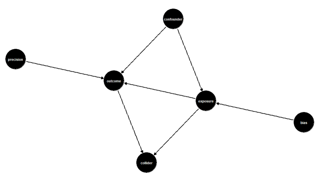
The confounding variables would be anything that affects both the exposure and the outcome. Other variables to include in the DAG are variables that impact only the outcome (precision variables) and variables that are descendants of both the exposure and the outcome (colliders). Variables that affect only the exposure can also be included in the DAG but should not be included in the analysis because they introduce bias into the model.
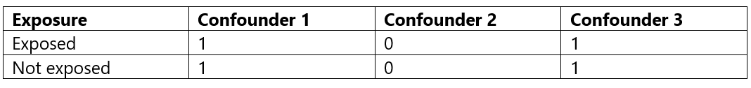
Once the DAG has been created, it’s time to start modeling. Matching is a modeling type that takes observations from each exposure that match across the remaining variables. For example, one observation would be exposed, and one would be unexposed, but all other variables would have the same value. These two observations would be considered “matched.” This allows the effect of the exposure to be measured directly without the impact of the confounders. The table below shows two matched variables as an example.
There are a few options to modify the matching process to better fit the dataset and context that is being used. First, there are many different matching types that can be used, from nearest neighbor to full matching. The “exact” parameter allows the specification for which variables should be matched on exact values as opposed to similar values. The function also allows the ratio of treated to untreated variables to be specified. This is useful when there are fewer exposed variables than unexposed, and an exposed variable may be matched to more than one unexposed variable.
Once the matched model has been created, the final step is to assess the results and determine an answer to the original question. One simple way to do this is to group the matched data on the exposure and calculate the mean outcome. This will display the mean effect that the exposure has on the outcome variable. In some cases, there may be suspicion that a particular group in a categorical confounder may be affected differently by the exposure than the overall population. In this case, those groups can be investigated by using the same result assessment as before, but with the added grouping of the variable of interest. This will break down the exposure effect further so that different groups can be compared.
By looking at these numbers, it can be determined whether the exposure has a positive or negative impact on the outcome, and how strong that impact is. These results can be used to inform action. In the case of our example, we might find that providing telehealth to a population improves the likelihood that a consumer received services within 14 days of their original assessment. If we wanted to drill down further, we could investigate this across age groups and find that telehealth improves this metric for teens even more than it does for the general population.
These results provide confidence in the effectiveness (or ineffectiveness) of an intervention to improve care or access to care. The results can inform the next course of action, whether that is to support intervention implementation or stop intervention implementation.
Propensity score modeling can provide a better understanding of interventions and their outcomes. This can help organizations make more informed decisions and ensure resources are allocated effectively. If you find yourself trying to understand a complex relationship between an exposure and an outcome, consider propensity score modeling as a solution.
Barrett, M., D’Agostino McGowan, L., Gerke, T. (2024, July 1). Causal Inference in R. Retrieved July 31, 2024, from https://www.r-causal.org/.
Valojerdi, A. E., & Janani, L. (2018, December 7). A brief guide to propensity score analysis. National Library of Medicine. National Library of Medicine (10.14196/mjiri.32.122).
matchit: Matching for Causal Inference (n.d.). RDocumentation. Retrieved August 7, 2024, from https://www.rdocumentation.org/packages/MatchIt/versions/4.5.5/topics/matchit.